Memory-Based Learning

The basic idea behind memory-based learning is that concepts can be classified by their similarity with previously seen concepts. In a memory-based system, learning amounts to storing the training data items. The strength of such a system lies in its capability to compute the similarity between a new data item and the training data items. The most simple similarity metric is the overlap metric [Daelemans et al.(2000)]. It compares corresponding features of the data items and adds 1 to a similarity rate when they are different. The similarity between two data items is represented by a number between zero and the number of features, $n$, in which value zero corresponds with an exact match and $n$ corresponds with two items which share no feature value. Here is an example:

TRAIN1	man	saw	the	V
TRAIN2	the	saw	.	N
TEST1	boy	saw	the	?

It contains two training items of a part-of-speech (POS) tagger and one test item for which we want to obtain a POS tag. Each item contains three features: the word that needs to be tagged (saw) and the preceding and the next word. In order to find the best POS tag for the test item, we compare its features with the features of the training data items. The test item shares two features with the first training data item and one with the second. The similarity value for the first training data item (1) is smaller than that of the second (2) and therefore the overlap metric will prefer the first.

A weakness of the overlap metric is that it regards all features as equally valuable for computing similarity values. Generally some features are more important than others. For example, when we add a line ``TRAIN3 boy and the C'' to our training data, the overlap metric will regard this new item as equally important as the first training item. Both the first and the third training item share two feature values with the test item but we would like the third to receive a lower similarity value because it does not contain the word for which we want find a POS tag (saw). In order to accomplish this, we assign weights to the features in such a way that the second feature receives a higher weight than the other two.

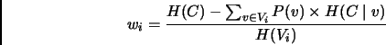
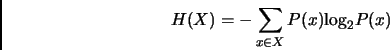
The method which we use to assign weights to the features is called Gain Ratio, a normalized variant of information gain [Daelemans et al.(2000)]. It estimates feature weights by examining the training data and determines for each feature how much information it contributes to the knowledge of the classes of the training data items. The weights are normalized in order to account for features with many different values. The Gain Ratio computation of the weights is summarized in the following formulas:

$$w_i = \frac{H(C)-\sum_{v\in V_i}P(v)\times H(C\mid v)}{H(V_i)}$$ (1)

$$H(X) = - \sum_{x\in X} P(x){\rm log}_2P(x)$$ (2)

Here $w_i$ is the weight of feature $i$, $C$ the set of class values and $V_i$ the set of values that feature $i$ can take. $H(C)$ and $H(V_i)$ are the entropy of the sets $C$ and $V_i$ respectively and $H(C\mid v)$ is the entropy of the subset of elements of $C$ that are associated with value $v$ of feature $i$. $P(v)$ is the probability that feature $i$ has value $v$. The normalization factor $H(V_i)$ was introduced to prevent that features with low generalization capacities, like identification codes, would obtain large weights.

The memory-based learning software which we have used in our experiments, TiMBL [Daelemans et al.(2000)], contains several algorithms with different parameters. In this paper we have restricted ourselves to using a single algorithm (k nearest neighbor classification) with a constant parameter setting. It would be interesting to evaluate every algorithm with all of its parameters but this would require a lot of extra work. We have changed only one parameter of the nearest neighbor algorithm from its default value: the size of the nearest neighborhood region. The learning algorithm computes the distance between the test item and the training items. The test item will receive the most frequent classification of the nearest training items (nearest neighborhood size is 1). [Daelemans et al.(1999)] show that using a larger neighborhood is harmful for classification accuracy for three language tasks but not for noun phrase chunking, a task which is central to this paper. In our experiments we have found that using the three nearest sets of data items leads to a better performance than using only the nearest data items. This increase of the neighborhood size used leads to a form of smoothing which can get rid of the influence of some data inconsistencies and exceptions.